Hydropower is one of the most commercially developed renewable energy sources globally. This study assessed the hydropower generation potential of the Pwalugu River section of the White Volta River in Ghana using the depth-averaged shallow-water equations (SWEs) hydrodynamic model. Various topographic models of the seabed were engineered to assess the topographic response to hydrodynamic flow, including the formation of whirlpools. The modelled equations were discretised using the Lax-Wendroff iteration scheme, and Python 3.07 was employed to implement the algorithm. The computed hydropower associated with the flowing fluid showed a significant difference before and after interacting with the engineered bottom-topographic structures. The topographic response to the flow led to increased mass flow rate, instigated by the developed flowing whirlpool, which served as a dynamic energy storage system for the flow channel. The topographic model with two mounts arranged along the river channel could produce power within the range of 1.8 MW - 2.9 MW. These were observed at locations x = 240 m, x = 481 m, and x = 962 m from the source of disturbances. The study, therefore, showed that the Pwalugu River section of White Volta River has the potential of generating hydropower if turbines are sited at these locations to enhance power generation capacity for the electrification of rural communities and the utlisation of the spillage from the Bagre dam in Burkina Faso, which causes perennial flooding in low-lying communities along the White Volta and the Black Volta in Ghana.
| Published in | Journal of Water Resources and Ocean Science (Volume 15, Issue 1) |
| DOI | 10.11648/j.wros.20261501.13 |
| Page(s) | 16-28 |
| Creative Commons |
This is an Open Access article, distributed under the terms of the Creative Commons Attribution 4.0 International License (http://creativecommons.org/licenses/by/4.0/), which permits unrestricted use, distribution and reproduction in any medium or format, provided the original work is properly cited. |
| Copyright |
Copyright © The Author(s), 2026. Published by Science Publishing Group |
Hydropower, Lax-Wendroff Scheme, Shallow Water Equation, Topographic Model, White Volta River
SWEs | Shallow Water Equations |
MW | Megawatt |
GW | Gigawatt |
kW | Kilowatt |
TWh | Terawatt-hour |
SHP | Small Hydropower Plant |
PDEs | Partial Differential Equations |
kWh | Kilowatt-Hour |
| [1] | G. A. Ryabov, “Cofiring of Coal and Fossil Fuels is a Way to Decarbonization of Heat and Electricity Generation (Review),” Thermal Engineering, vol. 69, no. 6, pp. 405–417, Jun. 2022, |
| [2] | L. Cherwoo et al., “Biofuels an alternative to traditional fossil fuels: A comprehensive review,” Sustainable Energy Technologies and Assessments, vol. 60, p. 103503, Dec. 2023, |
| [3] | Z. Li, S. Chen, and X. Chang, “Achieving clean energy via economic stability to qualify sustainable development goals in China,” Econ Anal Policy, vol. 81, pp. 1382–1394, Mar. 2024, |
| [4] | S. Penin y Santos, E. F. de Carvalho, and C. A. de S. Penin, “The Big Challenge: Reducing Global Emissions and Increasing Global GDP,” Journal of Electrical Power & Energy Systems, vol. 8, no. 2, pp. 76–93, Apr. 2025, |
| [5] | O. Abramova, “The Population of Africa under the Conditions of Transformation of the World Order,” Her Russ Acad Sci, vol. 92, no. S14, pp. S1306–S1315, Dec. 2022, |
| [6] | B. Mufutau Opeyemi, “Path to sustainable energy consumption: The possibility of substituting renewable energy for non-renewable energy,” Energy, vol. 228, p. 120519, Aug. 2021, |
| [7] | L. C. Voumik, Md. A. Islam, S. Ray, N. Y. Mohamed Yusop, and A. R. Ridzuan, “CO2 Emissions from Renewable and Non-Renewable Electricity Generation Sources in the G7 Countries: Static and Dynamic Panel Assessment,” Energies (Basel), vol. 16, no. 3, p. 1044, Jan. 2023, |
| [8] | A. Kumar and D. B. Pal, “Renewable Energy Development Sources and Technology: Overview,” Springer, Singapore, 2025, pp. 1–23. |
| [9] | A. A. K. Alhijazi, R. A. Almasri, and A. F. Alloush, “A Hybrid Renewable Energy (Solar/Wind/Biomass) and Multi-Use System Principles, Types, and Applications: A Review,” Sustainability, vol. 15, no. 24, p. 16803, Dec. 2023, |
| [10] | N. K. K. A. and V. A., “Renewable Energy Resources and Their Types,” IGI Global Scientific Publishing, 2023, pp. 116–135. |
| [11] | K. R. Abbasi, M. Shahbaz, J. Zhang, M. Irfan, and R. Alvarado, “Analyze the environmental sustainability factors of China: The role of fossil fuel energy and renewable energy,” Renew Energy, vol. 187, pp. 390–402, Mar. 2022, |
| [12] | S. O. Sanni, J. Y. Oricha, T. O. Oyewole, and F. I. Bawonda, “Analysis of backup power supply for unreliable grid using hybrid solar PV/diesel/biogas system,” Energy, vol. 227, p. 120506, Jul. 2021, |
| [13] | M. Muzammal Islam et al., “Improving Reliability and Stability of the Power Systems: A Comprehensive Review on the Role of Energy Storage Systems to Enhance Flexibility,” IEEE Access, vol. 12, pp. 152738–152765, 2024, |
| [14] | U. S. Bhatt, B. A. Carreras, J. M. R. Barredo, D. E. Newman, P. Collet, and D. Gomila, “The Potential Impact of Climate Change on the Efficiency and Reliability of Solar, Hydro, and Wind Energy Sources,” Land (Basel), vol. 11, no. 8, p. 1275, Aug. 2022, |
| [15] | National Renewable Energy Laboratory, “NREL Is Strengthening the Future of Hydropower, A Cornerstone of America’s Energy System,” 2025. Accessed: Dec. 29, 2025. [Online]. Available: |
| [16] | A. Wasti, P. Ray, S. Wi, C. Folch, M. Ubierna, and P. Karki, “Climate change and the hydropower sector: A global review,” Wiley Interdiscip Rev Clim Change, vol. 13, no. 2, p. e757, Mar. 2022, |
| [17] | H. E. Fälth, F. Hedenus, L. Reichenberg, and N. Mattsson, “Through energy droughts: Hydropower’s ability to sustain a high output,” Renewable and Sustainable Energy Reviews, vol. 214, p. 115519, May 2025, |
| [18] | A. Moulaye Abdou and A. Ahmed Abdou, “Multi Use Water System Approach for Small Hydro Power Plants (SHPP) alongside Irrigation and Drinking Water Supply (DWS) Networks,” in Advances in Hydropower Technologies, IntechOpen, 2024. |
| [19] | S. J. W. Klein and E. L. B. Fox, “A review of small hydropower performance and cost,” Renewable and Sustainable Energy Reviews, vol. 169, p. 112898, Nov. 2022, |
| [20] | U. Azimov and N. Avezova, “Sustainable small-scale hydropower solutions in Central Asian countries for local and cross-border energy/water supply,” Renewable and Sustainable Energy Reviews, vol. 167, p. 112726, Oct. 2022, |
| [21] | W. M. Tefera and K. S. Kasiviswanathan, “A global-scale hydropower potential assessment and feasibility evaluations,” Water Resour Econ, vol. 38, p. 100198, Apr. 2022, |
| [22] | A. Adu-Poku et al., “Impact of drought on hydropower generation in the Volta River basin and future projections under different climate and development pathways,” Energy and Climate Change, vol. 5, p. 100169, Dec. 2024, |
| [23] | B. E. Yankey et al., “Small hydropower development potential in the Densu River Basin, Ghana,” J Hydrol Reg Stud, vol. 45, p. 101304, Feb. 2023, |
| [24] | S. Nadarajah and C. Kwofie, “An extreme value analysis of water levels at the Akosombo dam, Ghana,” Heliyon, vol. 10, no. 14, p. e34076, Jul. 2024, |
| [25] |
Y. Song, C. Shen, and X. Liu, “A Surrogate Model for Shallow Water Equations Solvers with Deep Learning,” Journal of Hydraulic Engineering, vol. 149, no. 11, p. 04023045, Nov. 2023,
https://doi.org/10.1061/JHEND8.HYENG-13190;WGROUP:STRING:PUBLICATION |
| [26] | S. A. Rajput, S. A. Kamboh, K. B. Amur, and A. A. Bhutto, “Improved explicit finite difference method for extended shallow water partial differential equation,” Partial Differential Equations in Applied Mathematics, vol. 16, p. 101316, Dec. 2025, |
| [27] | A. I. Sukhinov, E. A. Protsenko, and S. V. Protsenko, “Comparative Analysis of Numerical and Analytical Studies of Hydrodynamic Processes in Shallow Water Bodies,” Water Resources, vol. 51, no. S2, pp. S216–S230, Dec. 2024, |
| [28] |
S. Hwang, B. Na, and S. Son, “Understanding Tidal Jet Vortices Over Complex Bathymetry via Numerical Modeling and Drone Observation: Match and Mismatch in the Vortex Dynamics Under Idealized and Realistic Topographic Settings,” J Geophys Res Oceans, vol. 129, no. 12, p. e2024JC021523, Dec. 2024,
https://doi.org/10.1029/2024JC021523;WGROUP:STRING:PUBLICATION |
| [29] | K. Nosrati, H. Afzalimehr, and J. Sui, “Interaction of Irregular Distribution of Submerged Rigid Vegetation and Flow within a Straight Pool,” Water (Basel), vol. 14, no. 13, p. 2036, Jun. 2022, |
| [30] | A. Ercan and M. L. Kavvas, “Self-similarity in incompressible Navier-Stokes equations,” Chaos, vol. 25, no. 12, Dec. 2015, |
| [31] |
L. Borzì et al., “Tsunami propagation and flooding maps: An application for the Island of Lampedusa, Sicily Channel, Italy,” Earth Surf Process Landf, vol. 49, no. 14, pp. 4842–4861, Nov. 2024,
https://doi.org/10.1002/ESP.5996;REQUESTEDJOURNAL:JOURNAL:10969837;WGROUP:STRING:PUBLICATION |
| [32] | C.-H. Lee, P. H.-Y. Lo, H. Shi, and Z. Huang, “Numerical Modeling of Generation of Landslide Tsunamis: A Review,” Journal of Earthquake and Tsunami, vol. 16, no. 06, Dec. 2022, |
| [33] | M. Y. Regina and E. S. Mohamed, “Modeling study of tsunami wave propagation,” International Journal of Environmental Science and Technology, vol. 20, no. 9, pp. 10491–10506, Sep. 2023, |
APA Style
Bowan, P. A., Kommiri, G., Musah, R. (2026). Hydropower Generation Potential of the Pwalugu River of the White Volta River Basin, Ghana. Journal of Water Resources and Ocean Science, 15(1), 16-28. https://doi.org/10.11648/j.wros.20261501.13
ACS Style
Bowan, P. A.; Kommiri, G.; Musah, R. Hydropower Generation Potential of the Pwalugu River of the White Volta River Basin, Ghana. J. Water Resour. Ocean Sci. 2026, 15(1), 16-28. doi: 10.11648/j.wros.20261501.13
@article{10.11648/j.wros.20261501.13,
  author = {Patrick Aaniamenga Bowan and Gerald Kommiri and Rabiu Musah},
  title = {Hydropower Generation Potential of the Pwalugu River of the White Volta River Basin, Ghana},
  journal = {Journal of Water Resources and Ocean Science},
  volume = {15},
  number = {1},
  pages = {16-28},
  doi = {10.11648/j.wros.20261501.13},
  url = {https://doi.org/10.11648/j.wros.20261501.13},
  eprint = {https://article.sciencepublishinggroup.com/pdf/10.11648.j.wros.20261501.13},
  abstract = {Hydropower is one of the most commercially developed renewable energy sources globally. This study assessed the hydropower generation potential of the Pwalugu River section of the White Volta River in Ghana using the depth-averaged shallow-water equations (SWEs) hydrodynamic model. Various topographic models of the seabed were engineered to assess the topographic response to hydrodynamic flow, including the formation of whirlpools. The modelled equations were discretised using the Lax-Wendroff iteration scheme, and Python 3.07 was employed to implement the algorithm. The computed hydropower associated with the flowing fluid showed a significant difference before and after interacting with the engineered bottom-topographic structures. The topographic response to the flow led to increased mass flow rate, instigated by the developed flowing whirlpool, which served as a dynamic energy storage system for the flow channel. The topographic model with two mounts arranged along the river channel could produce power within the range of 1.8 MW - 2.9 MW. These were observed at locations x = 240 m, x = 481 m, and x = 962 m from the source of disturbances. The study, therefore, showed that the Pwalugu River section of White Volta River has the potential of generating hydropower if turbines are sited at these locations to enhance power generation capacity for the electrification of rural communities and the utlisation of the spillage from the Bagre dam in Burkina Faso, which causes perennial flooding in low-lying communities along the White Volta and the Black Volta in Ghana.},
 year = {2026}
}
TY  - JOUR
T1  - Hydropower Generation Potential of the Pwalugu River of the White Volta River Basin, Ghana
AU  - Patrick Aaniamenga Bowan
AU  - Gerald Kommiri
AU  - Rabiu Musah
Y1  - 2026/02/04
PY  - 2026
N1  - https://doi.org/10.11648/j.wros.20261501.13
DO  - 10.11648/j.wros.20261501.13
T2  - Journal of Water Resources and Ocean Science
JF  - Journal of Water Resources and Ocean Science
JO  - Journal of Water Resources and Ocean Science
SP  - 16
EP  - 28
PB  - Science Publishing Group
SN  - 2328-7993
UR  - https://doi.org/10.11648/j.wros.20261501.13
AB  - Hydropower is one of the most commercially developed renewable energy sources globally. This study assessed the hydropower generation potential of the Pwalugu River section of the White Volta River in Ghana using the depth-averaged shallow-water equations (SWEs) hydrodynamic model. Various topographic models of the seabed were engineered to assess the topographic response to hydrodynamic flow, including the formation of whirlpools. The modelled equations were discretised using the Lax-Wendroff iteration scheme, and Python 3.07 was employed to implement the algorithm. The computed hydropower associated with the flowing fluid showed a significant difference before and after interacting with the engineered bottom-topographic structures. The topographic response to the flow led to increased mass flow rate, instigated by the developed flowing whirlpool, which served as a dynamic energy storage system for the flow channel. The topographic model with two mounts arranged along the river channel could produce power within the range of 1.8 MW - 2.9 MW. These were observed at locations x = 240 m, x = 481 m, and x = 962 m from the source of disturbances. The study, therefore, showed that the Pwalugu River section of White Volta River has the potential of generating hydropower if turbines are sited at these locations to enhance power generation capacity for the electrification of rural communities and the utlisation of the spillage from the Bagre dam in Burkina Faso, which causes perennial flooding in low-lying communities along the White Volta and the Black Volta in Ghana.
VL  - 15
IS  - 1
ER  -
Department of Civil Engineering, Dr. Hilla Limann Technical University, Wa, Ghana
Biography: Patrick Aaniamenga Bowan is an associate professor at Dr. Hilla Limann Technical University, Wa, Ghana, Department of Civil Engineering. He completed his PhD in Civil Engineering from Loughborough University, UK, in 2018, and obtained his Master's in Environmental Security from the University for Development Studies (UDS), Navrongo Campus, Ghana, in 2011. Recognised for his exceptional contributions, Prof Bowan has been honoured with the Senior Professional Engineer (SPE) designation by the Ghana Institution of Engineering (GhIE). In addition, he has been involved in consultancy services and currently serves on the Editorial Boards of numerous publications.
Research Fields: Water Science and Engineering, Environmental Engineering, Irrigation Engineering, Solid Waste Engineering and Management, Renewable Energy, Environmental Protection and Remediation, and Occupational Health and Safety.

Department of Mathematics, University for Development Studies, Tamale, Ghana
Biography: Gerald Kommiri is an MPhil Mathematics graduate of the Department of Mathematics, University for Development Studies, Tamale, Ghana and is currently a physics teacher at Notre Dame Minor Seminary School, Navrongo in Ghana. He is very passionate about studying fluid behaviour in hydropower generation.
Research Fields: Fluid flow, Mathematical modelling, Renewable Energy, Climate Change, and Water Resources Management.

Department of Electrical and Electronics Engineering, University for Development Studies, Tamale, Ghana
Biography: Rabiu Musah is a Senior Lecturer in the Department of Physics at the University for Development Studies (UDS), Nyankpala Campus, Ghana. He is known for his research in fluid dynamics, specifically MHD flow and nanofluids, with numerous publications and citations, serving as a key academic contributor in engineering and physics at the institution.
Research Fields: magnetohydrodynamics (MHD), Hybrid nanofluids, Flow Characteristics, Renewable and Blue Energy Modelling, and Computational and Mathematical Modelling.


Figure 1. A Shallow Water Channel with Irregular Bed Topography.
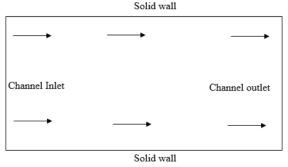
Figure 2. Computational Domain of River Channel.
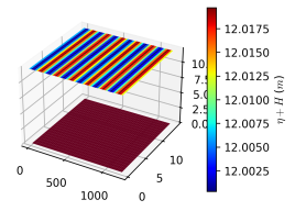
Figure 3. 3D flow pattern along a flat-bottom channel due to waves.
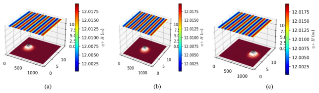
Figure 4. Locations of the bottom mountain at (a) channel entrance, (b) channel middle, (c) channel extreme.
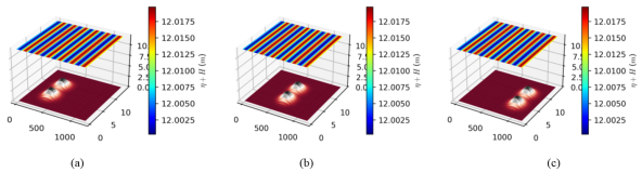
Figure 5. Location of the double bottom mountains model at (a) channel entrance, (b) channel middle, (c) channel end.
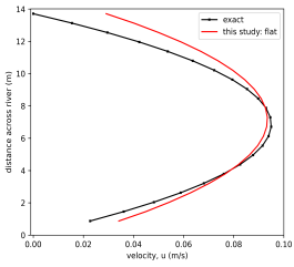
Figure 6. Comparison of the flow profile in an ideal channel with the model.
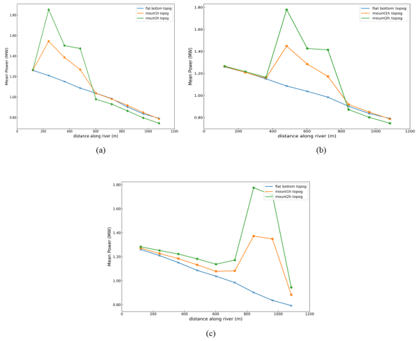
Figure 7. Graph of mean power along the river channel due to the bottom mountain at: (a) channel entrance, (b) channel middle, and (c) channel extreme.
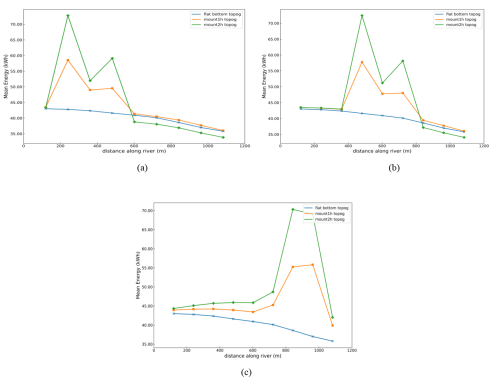
Figure 8. Graph of mean energy along the river channel due to the bottom mountain at (a) channel entrance, (b) channel middle, (c) channel extreme.
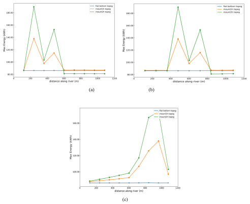
Figure 9. Graph of maximum energy along the river channel due to the bottom mountain at (a) channel entrance, (b) channel middle, (c) channel extreme.
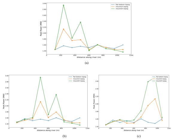
Figure 10. Graph of maximum power along the river channel due to the bottom mountain at (a) channel entrance, (b) channel middle, (c) channel extreme.